Vostok

Objective

One of the primary results of paleoclimate research over the past several decades has been strong evidence for human-influenced (anthropogenic) global warming. Results have been based on ice cores taken from undisturbed, ancient ice sheets, such as those in Antarctica. Ice cores provide uninterrupted information on important properties of paleoclimate, including local temperature and precipitation rate, humidity, and wind speed as well as changes in atmospheric composition of dust and gases. Remember that climate is the long-term average of weather; that is, short term variations in temperature and precipitation such as individual storms, are averaged together to give the long-term values of climate. Consider that you have been chosen and funded by Congress as one of the scientists who will participate in analyzing the latest of these ice cores (it might have also been a desire of yours to go to Antarctica!). Politicians as well as scientists and the general public are interested in determining whether the warming we see today was really caused by humans or is it just natural variability that is part Earth’s system of the distant, geological past. In this lab we will work with the original data from the famous Vostok Ice Cores, which carry the distinction of being the only ice cores that scientists are certain have remained undisturbed for the last interglacial and the penultimate glacial periods.

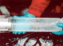
Figure 1

Ice core

Vostok is the Antarctic research base founded by the Soviet Union in 1957. Even though the US has bragging rights to a research base at the South Pole, the (now) Russian base at Vostok is much more important scientifically. First of all it sits over one of the thickest (>4km) portions of the East Antarctic Ice Sheet. Second, this ice is relatively undisturbed (elsewhere the ice has been subject to substantial flow and/or seasonal conditions that might destroy the ice). Third, under the 4km ice sheet at Vostok lies a lake the size of Lake Ontario that has been cut off from Earth surface conditions for perhaps 15 million years. In a recent, exciting scientific advance reserachers recently drilled through the last bit of ice and have made contact with the lake water.

Figure 2

Antarctica with Lake Vostok circled

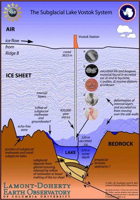
Figure 3

The subglacial Lake Vostok system

Part 1. Ice and Gas Ages in the Vostok Core

NOTE: It is by far easiest to do this lab in the Microsoft EXCEL program. The University offers this program as part of the Microsoft Office 365 package (includes Word and Powerpoint) to all students for free. To get the software start at the following link and go through the instructions: https://documentation.its.umich.edu/node/2328

In addition, for those who are new to Excel there is a brief "Excel_primer.xlsx" file that is available on \Canvas\Lab_Resources. This file provides information on the basics of using Excel, including how to make graphs and calculate regressions. Information on these operations will be useful for this lab.

Open the Excel file entitled totalvosdata.xls. Click on the "Vostok" tab of the excel sheet. This dataset contains columns that give the depth (in meters) of the ice core, the "ice" and "gas" ages (in thousands of years ago), concentrations of carbon dioxide and methane found in the ice bubbles, the hydrogen isotopic ratios ("delta D"), and a column that provides information on dust.

The ice age (i.e., the age of the ice, not to be confused with our other use of the term ice age, which refers to a time in geologic history of pronounced glaciation) is obtained by counting layers of ice and, when layers are no longer clearly visible, modeling the flow of merged ice layers.

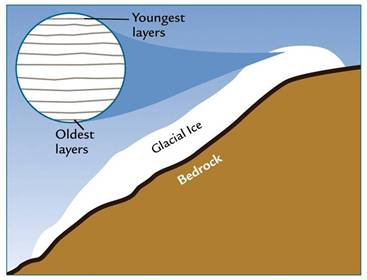
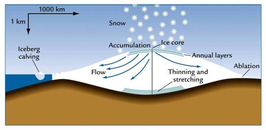
Figure 4 Figure 5

Annual ice layers Continental ice sheets

The gas age is calculated assuming that the bubbles of gas can only be trapped effectively in layers of older ice (i.e., at a depth well below the surface, where the pores in the ice close, sealing the air). This process is called sintering.

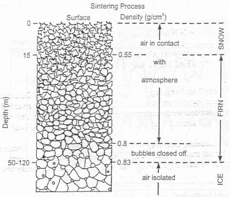
Figure 6

Sintering process - Raynaud, 1992

Plot both the ice age and the gas age as a function of depth. To do this: first, select the entire depth column by clicking on the "A" at the top of it, then hold down the control key (command on Macs) and select the ice age column by clicking on the "B" at the top, and then hold down the control key (command on Macs) and select the gas age column by clicking on the "E" at the top. Once all three columns are selected, click on the "Insert" tab, and insert a "Scatter with Straight Lines" plot. Now, right click on the graph and click "Select Data." Change series names to "Ice Age" and "Gas Age," respectively. Now click "OK" to generate the graph. Give your chart appropriate labels for the title and axes and also add a legend: axes labels, titles, and legends can be found under the "Chart Design" tab. Be sure to label the appropriate units. If you don't know what they should be, then re-read this lab again from the beginning. You should always know what you are graphing and why!

Question 1
The two age curves differ - why? How much younger, roughly, is a bubble of gas than the ice that surrounds it, at a depth of 1000 meters? (Hint: for this part you may need to look at the raw data for 1000 meters instead of your graph) Be sure to include your complete graph in the assignment you turn in.

Part 2. The Temperature Record

The temperature of the environment when the ice or sediment in a core was deposited can be estimated using isotopes of hydrogen or oxygen. The Vostok record is most complete for the hydrogen isotopes, but the concepts of understanding how the isotope-temperature relationship works is easier with oxygen. In addition, oxygen can be used to determine temperatures from ocean sediment cores as well.

Oxygen has two stable isotopes of importance, ¹⁶O and ¹⁸O, which vary in mass. Differences in the amounts of these isotopes in a sample (air, water, ice, rocks, organisms) are measured by comparing the ratio of ¹⁸O/¹⁶O in a sample to that ratio in a standard, which for oxygen is average ocean water. This comparison is called d¹⁸O (pronounced delta-18-O).

Variations in the d¹⁸O of the oxygen in the water molecule, H₂O, can be useful in understanding the hydrological cycle and the cycle of glaciations. Average ocean water has a value of 0‰ d¹⁸O (‰ is pronounced permil and is the symbol for one-thousandth. It is analogous to %, percent, which is the symbol for one-hundredth).

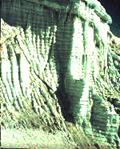
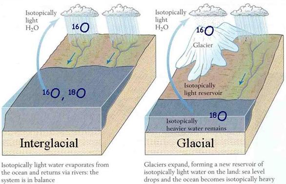
Figure 7 Figure 8

Layers of ice Isotopic signature during glacial and interglacial periods

When ocean water evaporates, water with the lighter oxygen isotope (¹⁶O) evaporates more easily because it is lighter than a water molecule with the heavier oxygen isotope (¹⁸O). Therefore, water vapor in the atmosphere ends up with a smaller percentage of ¹⁸O in it than ocean water. Its d¹⁸O is a few permil negative, say around –3‰. When that vapor passes over land and condenses to form rain, the heavier isotopes that did make it into the clouds condense to a greater extent than the lighter isotopes, again due to mass. Precipitation that falls then has a more negative d¹⁸O than seawater, but more positive d¹⁸O than the clouds from which it fell. This effect is more pronounced in cold climates than in warmer ones, because temperature is what drives the evaporation/condensation processes. Snow has much more negative d¹⁸O than rain. Because temperature drives this process, an equation can be derived to relate temperature to d¹⁸O (or Hydrogen). Therefore, times of glaciation are associated with more negative d¹⁸O in ice samples.

Now let's make the transition to hydrogen, because H isotopes are what you will work with in this lab (and, it was the first data, before oxygen, to be produced from the ice cores). The hydrogen isotopes of interest to paleoclimate studies are ¹H and ²H. The fractionation of heavy and light hydrogen isotopes behaves similiarly to oxygen isotopes. Since ²H is such an important isotope to nuclear chemistry, it has its own name: Deuterium. Both oxygen and hydrogen isotopic fractionation can be related to temperature (and thus if you have one you can relate it to the other), and in this lab, we use the hydrogen isotopes.

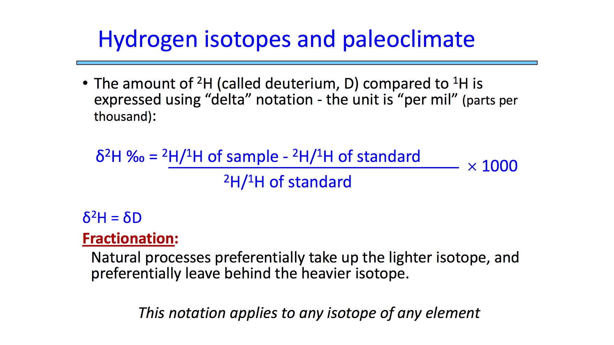
Figure 9 Lecture Figure

Structure of Deuterium Hydrogen Isotopes and Paleoclimate

We want to convert the deuterium isotopic ratios to temperature changes (delta temperatures) that describe variations in the temperature of the ocean from which the ice was originally evaporated. This has been determined by past studies, and you can reproduce this equation in Excel by doing the following: Type delta temp in the first row of a new column (column H), and deg C in the second row of the same column. Now use Excel to calculate the delta temperatures, filling in your new column, by using the instructions below. Note that the "delta temperature" is relative to the current temperature today.

Use the following conversion factor that is derived from the relationship between the deuterium value and air temperature (as shown in lecture). Type: =(C3 + 440)/6.2 into the third cell of column H ("delta temp") and press Enter (return on Macs). (Make sure you include the equals sign when typing the equation into the cell.) Then click on that same cell again and put the cursor on the lower right corner of it until it turns into a black cross. Click and hold on the black cross and drag down to the end of the column (while still holding down). The cross cursor applies the relationship of the first cell to other cells. (To make sure it worked, check and see if the numbers in each row are different. If they are all the same, it didn't work.) Highlight the column (right-click on the "H" at the top), click "Format Cells", and give the numbers two decimal places.

Figure 10

Drilling ice cores at Vostok

Save your work. Think about why the delta temperatures change with deuterium isotope ratio in the way they do. If you don't understand, then you should be sure to read through the suggested readings listed at the end of this lab and look at the web notes for the lecture on Climate Change and the Ice Ages on Canvas, Lecture Schedule.

Question 2
Plot the delta temperature curve as a function of ice age (ice age is on the X axis; use a "Scatter with Straight Lines" graph) and copy it into your report. How many degrees of temperature has climate varied in the past, as indicated in these data? Over what time scale can a shift from minimum to maximum temperature occur? Be sure to include your graph in the assignment you turn in.

Question 3
According to your graph, approximately when did the last period of full glacial conditions begin and end (no transition zones)? When did the current interglacial conditions (temperatures) begin and end? Be sure to include your graph in the assignment you turn in.

Part 3. The Atmospheric Composition and Dust Record

Another piece of information that comes from ice cores is the amount of dust that was in the atmosphere. During the last ice age, sea level was 100-120 meters lower and much more land was exposed. In addition, it was much colder, and that had an effect on the distribution of vegetation. In this section, you will put together the different pieces of information that come from the core. Use the following graphs of CO₂ and CH₄ concentration, as well as delta temperature and dust as a function of age, to answer the questions for this section.

Figure 11

Carbon dioxide and methane concentrations plotted with delta temperature

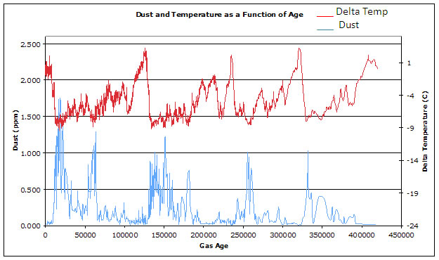
Figure 12

Dust (lower curve, blue) and temperature (upper curve, red) as a function of age

Question 4
Note the time of the major warming events. Then look at how CO₂ and CH₄ change during the same time. Referring to Figure 11 (above), can you tell which changes first, temperature or greenhouse gas (CO₂, CH₄) composition? (Note the direction of the x-axis.) Explain the pattern you see in the graph and explain what is causing the pattern or why it is happening.

Question 5
Referring to Figure 12 (above), why were dust concentrations different during the glacial and interglacial periods?

Part 4. What can we learn from this analysis of past climate about climate on earth today?

Now we will reproduce the steps necessary to convert the isotope data to the air temperature of the past. First add another column to your Excel file to estimate the temperature at Vostok. Label the column "Vostok Temp. (deg C)". To do this, subtract 55.5 degrees from the numbers in the delta temperature column to get an estimate of the Vostok air temperature itself.

Create scatter plots (without connecting lines) of CO₂ (x-axis) vs. temperature (y-axis) and CH₄ (x-axis) vs. temperature (y-axis) using the Vostok data. Change the minimum and maximum values of your x and y axes to appropriately display the data. Insert a linear "trendline" (which is found under the Chart Design tab) and report the equation and R² value by checking those boxes in the option menu for trendlines of each scatter plot in your lab report. The R-squared (R²) is a statistical measure of how well actual data fit a linear regression model (note: the R² is NOT the radius squared and is NOT the inverse-square law); an R-squared of 1.0 (100%) indicates a perfect fit of the data to a straight line. So if you had an R² of 1.0 for the CO₂ vs. temperature plot, if you knew the CO₂ concentration you could predict the corresponding temperature 100% of the time (in the real world, very few relationships are 100% perfect).

Question 6
Copy your scatter plots with trendlines into your report. Why is the R² value for CO₂ or CH₄ less than one? In other words, explain why the relationships are not perfect fits (the fit of the trendline to the data is not perfect, there are points that do not lie right on the trendline).

Question 7
Predict the temperature at Vostok today. Use the current, average, CO₂ concentration (400 ppmv) to solve the linear regression equation from the past relationship between CO₂ and temperature (Q6). How does this calculated temperature differ from the surface temperature today at Vostok? Explain why these may be different. (You can look up this temperature with a weather website - this will give you a temperature in Farenheit, and you want it in Celsius.) Remember to consider the difference between weather and climate.

Please submit a Word document on Canvas containing answer to questions 1 through 7 and graphs (with titles and axis labels) for questions 1, 2, and 6.

Sources

Monnin et al. "Atmospheric CO2 concentrations over
the last glacial termination" Science v.291, 112-114, 5 January 2001.

Dansgaard, W., H.B. Clausen, N. Gundestrup, C. U. Hammer, S. J. Johnsen, P. M. Kristinsdottir, and N. Reeh, A New Greenland Deep Ice Core, Science, Vol. 218, 1992, p.1273-1277.

"Deciphering Mysteries of Past Climate From Antarctic Ice Cores" Earth in Space (American Geophysical Union), Vol. 8, No. 3, November 1995, p. 9.

Crane, Robert G., James F. Kasting, and Lee R. Kump. The Earth System. New Jersey: Prentice Hall, 1999.

http://www.aad.gov.au/asset/images/525_ul-core.jpg

A great source of paleoclimatological data can be found at the NOAA web site.

Back to index